STARKs, Part II: Thank Goodness It's FRI-day
2017 Nov 22
See all posts
STARKs, Part II: Thank Goodness It's FRI-day
Special thanks to Eli Ben-Sasson for ongoing help and explanations, and Justin Drake for reviewing
In the last part of this series, we talked about how you can make some pretty interesting succinct proofs of computation, such as proving that you have computed the millionth Fibonacci number, using a technique involving polynomial composition and division. However, it rested on one critical ingredient: the ability to prove that at least the great majority of a given large set of points are on the same low-degree polynomial. This problem, called "low-degree testing", is perhaps the single most complex part of the protocol.
We'll start off by once again re-stating the problem. Suppose that you have a set of points, and you claim that they are all on the same polynomial, with degree less than \(D\) (ie. \(deg < 2\) means they're on the same line, \(deg < 3\) means they're on the same line or parabola, etc). You want to create a succinct probabilistic proof that this is actually true.
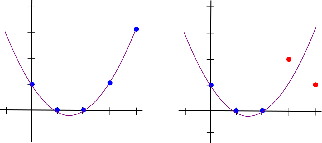
Left: points all on the same \(deg < 3\) polynomial. Right: points not on the same \(deg < 3\) polynomial
If you want to verify that the points are all on the same degree \(< D\) polynomial, you would have to actually check every point, as if you fail to check even one point there is always some chance that that point will not be on the polynomial even if all the others are. But what you can do is probabilistically check that at least some fraction (eg. 90%) of all the points are on the same polynomial.


Top left: possibly close enough to a polynomial. Top right: not close enough to a polynomial. Bottom left: somewhat close to two polynomials, but not close enough to either one. Bottom right: definitely not close enough to a polynomial.
If you have the ability to look at every point on the polynomial, then the problem is easy. But what if you can only look at a few points - that is, you can ask for whatever specific point you want, and the prover is obligated to give you the data for that point as part of the protocol, but the total number of queries is limited? Then the question becomes, how many points do you need to check to be able to tell with some given degree of certainty?
Clearly, \(D\) points is not enough. \(D\) points are exactly what you need to uniquely define a degree \(< D\) polynomial, so any set of points that you receive will correspond to some degree \(< D\) polynomial. As we see in the figure above, however, \(D+1\) points or more do give some indication.
The algorithm to check if a given set of values is on the same degree \(< D\) polynomial with \(D+1\) queries is not too complex. First, select a random subset of \(D\) points, and use something like Lagrange interpolation (search for "Lagrange interpolation" here for a more detailed description) to recover the unique degree \(< D\) polynomial that passes through all of them. Then, randomly sample one more point, and check that it is on the same polynomial.

Note that this is only a proximity test, because there's always the possibility that most points are on the same low-degree polynomial, but a few are not, and the \(D+1\) sample missed those points entirely. However, we can derive the result that if less than 90% of the points are on the same degree \(< D\) polynomial, then the test will fail with high probability. Specifically, if you make \(D+k\) queries, and if at least some portion \(p\) of the points are not on the same polynomial as the rest of the points, then the test will only pass with probability \((1 - p)^k\).
But what if, as in the examples from the previous article, \(D\) is very high, and you want to verify a polynomial's degree with less than \(D\) queries? This is, of course, impossible to do directly, because of the simple argument made above (namely, that any \(k \leq D\) points are all on at least one degree \(< D\) polynomial). However, it's quite possible to do this indirectly by providing auxiliary data, and achieve massive efficiency gains by doing so. And this is exactly what new protocols like FRI ("Fast RS IOPP", RS = "Reed-Solomon", IOPP = "Interactive Oracle Proofs of Proximity"), and similar earlier designs called probabilistically checkable proofs of proximity (PCPPs), try to achieve.
A First Look at Sublinearity
To prove that this is at all possible, we'll start off with a relatively simple protocol, with fairly poor tradeoffs, but that still achieves the goal of sublinear verification complexity - that is, you can prove proximity to a degree \(< D\) polynomial with less than \(D\) queries (and, for that matter, less than \(O(D)\) computation to verify the proof).
The idea is as follows. Suppose there are N points (we'll say \(N\) = 1 billion), and they are all on a degree \(<\) 1,000,000 polynomial \(f(x)\). We find a bivariate polynomial (ie. an expression like \(1 + x + xy + x^5 \cdot y^3 + x^{12} + x \cdot y^{11}\)), which we will denote \(g(x, y)\), such that \(g(x, x^{1000}) = f(x)\). This can be done as follows: for the \(k\)th degree term in \(f(x)\) (eg. \(1744 \cdot x^{185423}\)), we decompose it into \(x^{k \% 1000} \cdot y^{floor(k / 1000)}\) (in this case, \(1744 \cdot x^{423} \cdot y^{185}\)). You can see that if \(y = x^{1000}\), then \(1744 \cdot x^{423} \cdot y^{185}\) equals \(1744 \cdot x^{185423}\).
In the first stage of the proof, the prover commits to (ie. makes a Merkle tree of) the evaluation of \(g(x, y)\) over the entire square \([1 ... N] x \{x^{1000}: 1 \leq x \leq N\}\) - that is, all 1 billion \(x\) coordinates for the columns, and all 1 billion corresponding thousandth powers for the \(y\) coordinates of the rows. The diagonal of the square represents the values of \(g(x, y)\) that are of the form \(g(x, x^{1000})\), and thus correspond to values of \(f(x)\).
The verifier then randomly picks perhaps a few dozen rows and columns (possibly using the Merkle root of the square as a source of pseudorandomness if we want a non-interactive proof), and for each row or column that it picks the verifier asks for a sample of, say, 1010 points on the row and column, making sure in each case that one of the points demanded is on the diagonal. The prover must reply back with those points, along with Merkle branches proving that they are part of the original data committed to by the prover. The verifier checks that the Merkle branches match up, and that the points that the prover provides actually do correspond to a degree-1000 polynomial.

This gives the verifier a statistical proof that (i) most rows are populated mostly by points on degree \(< 1000\) polynomials, (ii) most columns are populated mostly by points on degree \(< 1000\) polynomials, and (iii) the diagonal line is mostly on these polynomials. This thus convinces the verifier that most points on the diagonal actually do correspond to a degree \(< 1,000,000\) polynomial.
If we pick thirty rows and thirty columns, the verifier needs to access a total of 1010 points \(\cdot\) 60 rows+cols = 60600 points, less than the original 1,000,000, but not by that much. As far as computation time goes, interpolating the degree \(< 1000\) polynomials will have its own overhead, though since polynomial interpolation can be made subquadratic the algorithm as a whole is still sublinear to verify. The prover complexity is higher: the prover needs to calculate and commit to the entire \(N \cdot N\) rectangle, which is a total of \(10^{18}\) computational effort (actually a bit more because polynomial evaluation is still superlinear). In all of these algorithms, it will be the case that proving a computation is substantially more complex than just running it; but as we will see the overhead does not have to be that high.
A Modular Math Interlude
Before we go into our more complex protocols, we will need to take a bit of a digression into the world of modular arithmetic. Usually, when we work with algebraic expressions and polynomials, we are working with regular numbers, and the arithmetic, using the operators +, -, \(\cdot\), / (and exponentiation, which is just repeated multiplication), is done in the usual way that we have all been taught since school: \(2 + 2 = 4\), \(72 / 5 = 14.4\), \(1001 \cdot 1001 = 1002001\), etc. However, what mathematicians have realized is that these ways of defining addition, multiplication, subtraction and division are not the only self-consistent ways of defining those operators.
The simplest example of an alternate way to define these operators is modular arithmetic, defined as follows. The % operator means "take the remainder of": \(15 % 7 = 1\), \(53 % 10 = 3\), etc (note that the answer is always non-negative, so for example \(-1 % 10 = 9\)). For any specific prime number \(p\), we can redefine:
\(x + y \Rightarrow (x + y)\) % \(p\)
\(x \cdot y \Rightarrow (x \cdot y)\) % \(p\)
\(x^y \Rightarrow (x^y)\) % \(p\)
\(x - y \Rightarrow (x - y)\) % \(p\)
\(x / y \Rightarrow (x \cdot y ^{p-2})\) % \(p\)
The above rules are all self-consistent. For example, if \(p = 7\), then:
- \(5 + 3 = 1\) (as \(8\) % \(7 = 1\))
- \(1 - 3 = 5\) (as \(-2\) % \(7 = 5\))
- \(2 \cdot 5 = 3\)
- \(3 / 5 = 2\) (as (\(3 \cdot 5^5\)) % \(7 = 9375\) % \(7 = 2\))
More complex identities such as the distributive law also hold: \((2 + 4) \cdot 3\) and \(2 \cdot 3 + 4 \cdot 3\) both evaluate to \(4\). Even formulas like \((a^2 - b^2)\) = \((a - b) \cdot (a + b)\) are still true in this new kind of arithmetic. Division is the hardest part; we can't use regular division because we want the values to always remain integers, and regular division often gives non-integer results (as in the case of \(3/5\)). The funny \(p-2\) exponent in the division formula above is a consequence of getting around this problem using Fermat's little theorem, which states that for any nonzero \(x < p\), it holds that \(x^{p-1}\) % \(p = 1\). This implies that \(x^{p-2}\) gives a number which, if multiplied by \(x\) one more time, gives \(1\), and so we can say that \(x^{p-2}\) (which is an integer) equals \(\frac{1}{x}\). A somewhat more complicated but faster way to evaluate this modular division operator is the extended Euclidean algorithm, implemented in python here.
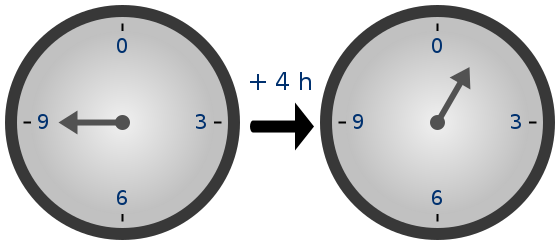
Because of how the numbers "wrap around", modular arithmetic is sometimes called "clock math"
With modular math we've created an entirely new system of arithmetic, and because it's self-consistent in all the same ways traditional arithmetic is self-consistent we can talk about all of the same kinds of structures over this field, including polynomials, that we talk about in "regular math". Cryptographers love working in modular math (or, more generally, "finite fields") because there is a bound on the size of a number that can arise as a result of any modular math calculation - no matter what you do, the values will not "escape" the set \(\{0, 1, 2 ... p-1\}\).
Fermat's little theorem also has another interesting consequence. If \(p-1\) is a multiple of some number \(k\), then the function \(x \rightarrow x^k\) has a small "image" - that is, the function can only give \(\frac{p-1}{k} + 1\) possible results. For example, \(x \rightarrow x^2\) with \(p=17\) has only 9 possible results.

With higher exponents the results are more striking: for example, \(x \rightarrow x^8\) with \(p=17\) has only 3 possible results. And of course, \(x \rightarrow x^{16}\) with \(p=17\) has only 2 possible results: for \(0\) it returns \(0\), and for everything else it returns \(1\).
Now A Bit More Efficiency
Let us now move on to a slightly more complicated version of the protocol, which has the modest goal of reducing the prover complexity from \(10^{18}\) to \(10^{15}\), and then \(10^{9}\). First, instead of operating over regular numbers, we are going to be checking proximity to polynomials as evaluated with modular math. As we saw in the previous article, we need to do this to prevent numbers in our STARKs from growing to 200,000 digits anyway. Here, however, we are going to use the "small image" property of certain modular exponentiations as a side effect to make our protocols far more efficient.
Specifically, we will work with \(p =\) 1,000,005,001. We pick this modulus because (i) it's greater than 1 billion, and we need it to be at least 1 billion so we can check 1 billion points, (ii) it's prime, and (iii) \(p-1\) is an even multiple of 1000. The exponentiation \(x^{1000}\) will have an image of size 1,000,006 - that is, the exponentiation can only give 1,000,006 possible results.
This means that the "diagonal" (\(x\), \(x^{1000}\)) now becomes a diagonal with a wraparound; as \(x^{1000}\) can only take on 1,000,006 possible values, we only need 1,000,006 rows. And so, the full evaluation of \(g(x, x^{1000})\) now has only ~\(10^{15}\) elements.
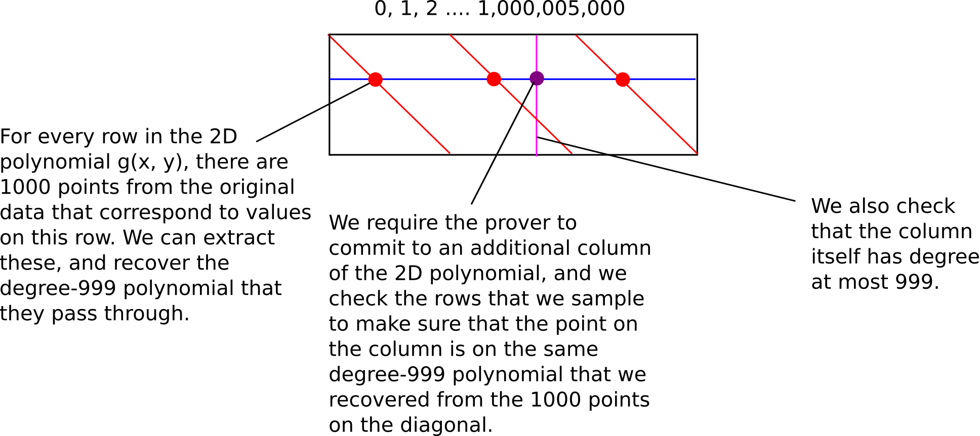
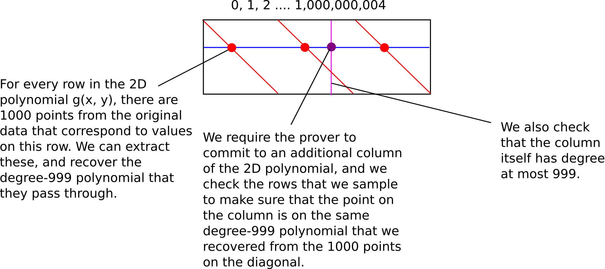
As it turns out, we can go further: we can have the prover only commit to the evaluation of \(g\) on a single column. The key trick is that the original data itself already contains 1000 points that are on any given row, so we can simply sample those, derive the degree \(< 1000\) polynomial that they are on, and then check that the corresponding point on the column is on the same polynomial. We then check that the column itself is \(a < 1000\) polynomial.
The verifier complexity is still sublinear, but the prover complexity has now decreased to \(10^9\), making it linear in the number of queries (though it's still superlinear in practice because of polynomial evaluation overhead).
And Even More Efficiency
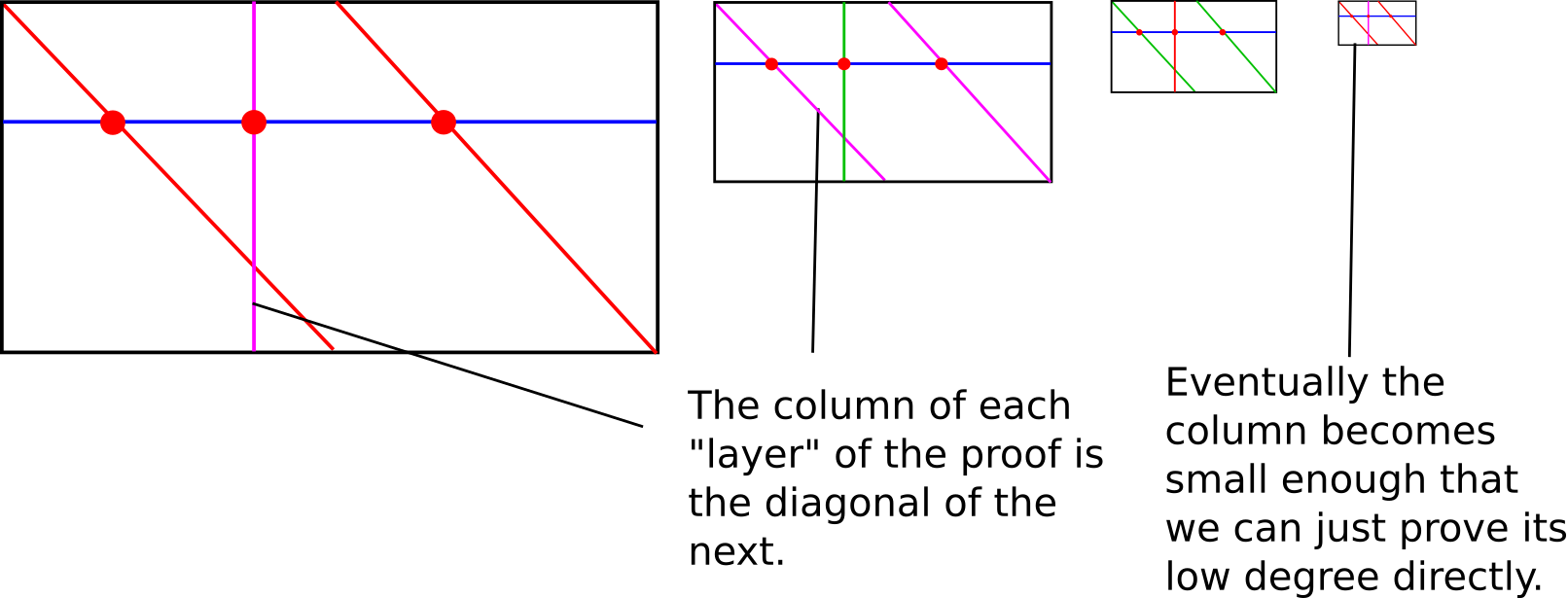
The prover complexity is now basically as low as it can be. But we can still knock the verifier complexity down further, from quadratic to logarithmic. And the way we do that is by making the algorithm recursive. We start off with the last protocol above, but instead of trying to embed a polynomial into a 2D polynomial where the degrees in \(x\) and \(y\) are equal, we embed the polynomial into a 2D polynomial where the degree bound in \(x\) is a small constant value; for simplicity, we can even say this must be 2. That is, we express \(f(x) = g(x, x^2)\), so that the row check always requires only checking 3 points on each row that we sample (2 from the diagonal plus one from the column).
If the original polynomial has degree \(< n\), then the rows have degree \(< 2\) (ie. the rows are straight lines), and the column has degree \(< \frac{n}{2}\). Hence, what we now have is a linear-time process for converting a problem of proving proximity to a polynomial of degree \(< n\) into a problem of proving proximity to a polynomial of degree \(< \frac{n}{2}\). Furthermore, the number of points that need to be committed to, and thus the prover's computational complexity, goes down by a factor of 2 each time (Eli Ben-Sasson likes to compare this aspect of FRI to fast fourier transforms, with the key difference that unlike with FFTs, each step of recursion only introduces one new sub-problem instead of branching out into two). Hence, we can simply keep using the protocol on the column created in the previous round of the protocol, until the column becomes so small that we can simply check it directly; the total complexity is something like \(n + \frac{n}{2} + \frac{n}{4} + ... \approx 2n\).
In reality, the protocol will need to be repeated several times, because there is still a significant probability that an attacker will cheat one round of the protocol. However, even still the proofs are not too large; the verification complexity is logarithmic in the degree, though it goes up to \(\log ^{2}n\) if you count the size of the Merkle proofs.
The "real" FRI protocol also has some other modifications; for example, it uses a binary Galois field (another weird kind of finite field; basically, the same thing as the 12th degree extension fields I talk about here, but with the prime modulus being 2). The exponent used for the row is also typically 4 and not 2. These modifications increase efficiency and make the system friendlier to building STARKs on top of it. However, these modifications are not essential to understanding how the algorithm works, and if you really wanted to, you could definitely make STARKs with the simple modular math-based FRI described here too.
Soundness
I will warn that calculating soundness - that is, determining just how low the probability is that an optimally generated fake proof will pass the test for a given number of checks - is still somewhat of a "here be dragons" area in this space. For the simple test where you take 1,000,000 \(+ k\) points, there is a simple lower bound: if a given dataset has the property that, for any polynomial, at least portion p of the dataset is not on the polynomial, then a test on that dataset will pass with at most \((1-p)^k\) probability. However, even that is a very pessimistic lower bound - for example, it's not possible to be much more than 50% close to two low-degree polynomials at the same time, and the probability that the first points you select will be the one with the most points on it is quite low. For full-blown FRI, there are also complexities involving various specific kinds of attacks.
Here is a recent article by Ben-Sasson et al describing soundness properties of FRI in the context of the entire STARK scheme. In general, the "good news" is that it seems likely that in order to pass the \(D(x) \cdot Z(x) = C(P(x))\) check on the STARK, the \(D(x)\) values for an invalid solution would need to be "worst case" in a certain sense - they would need to be maximally far from any valid polynomial. This implies that we don't need to check for that much proximity. There are proven lower bounds, but these bounds would imply that an actual STARK need to be ~1-3 megabytes in size; conjectured but not proven stronger bounds reduce the required number of checks by a factor of 4.
The third part of this series will deal with the last major part of the challenge in building STARKs: how we actually construct constraint checking polynomials so that we can prove statements about arbitrary computation, and not just a few Fibonacci numbers.
STARKs, Part II: Thank Goodness It's FRI-day
2017 Nov 22 See all postsSpecial thanks to Eli Ben-Sasson for ongoing help and explanations, and Justin Drake for reviewing
In the last part of this series, we talked about how you can make some pretty interesting succinct proofs of computation, such as proving that you have computed the millionth Fibonacci number, using a technique involving polynomial composition and division. However, it rested on one critical ingredient: the ability to prove that at least the great majority of a given large set of points are on the same low-degree polynomial. This problem, called "low-degree testing", is perhaps the single most complex part of the protocol.
We'll start off by once again re-stating the problem. Suppose that you have a set of points, and you claim that they are all on the same polynomial, with degree less than \(D\) (ie. \(deg < 2\) means they're on the same line, \(deg < 3\) means they're on the same line or parabola, etc). You want to create a succinct probabilistic proof that this is actually true.
Left: points all on the same \(deg < 3\) polynomial. Right: points not on the same \(deg < 3\) polynomial
If you want to verify that the points are all on the same degree \(< D\) polynomial, you would have to actually check every point, as if you fail to check even one point there is always some chance that that point will not be on the polynomial even if all the others are. But what you can do is probabilistically check that at least some fraction (eg. 90%) of all the points are on the same polynomial.
Top left: possibly close enough to a polynomial. Top right: not close enough to a polynomial. Bottom left: somewhat close to two polynomials, but not close enough to either one. Bottom right: definitely not close enough to a polynomial.
If you have the ability to look at every point on the polynomial, then the problem is easy. But what if you can only look at a few points - that is, you can ask for whatever specific point you want, and the prover is obligated to give you the data for that point as part of the protocol, but the total number of queries is limited? Then the question becomes, how many points do you need to check to be able to tell with some given degree of certainty?
Clearly, \(D\) points is not enough. \(D\) points are exactly what you need to uniquely define a degree \(< D\) polynomial, so any set of points that you receive will correspond to some degree \(< D\) polynomial. As we see in the figure above, however, \(D+1\) points or more do give some indication.
The algorithm to check if a given set of values is on the same degree \(< D\) polynomial with \(D+1\) queries is not too complex. First, select a random subset of \(D\) points, and use something like Lagrange interpolation (search for "Lagrange interpolation" here for a more detailed description) to recover the unique degree \(< D\) polynomial that passes through all of them. Then, randomly sample one more point, and check that it is on the same polynomial.
Note that this is only a proximity test, because there's always the possibility that most points are on the same low-degree polynomial, but a few are not, and the \(D+1\) sample missed those points entirely. However, we can derive the result that if less than 90% of the points are on the same degree \(< D\) polynomial, then the test will fail with high probability. Specifically, if you make \(D+k\) queries, and if at least some portion \(p\) of the points are not on the same polynomial as the rest of the points, then the test will only pass with probability \((1 - p)^k\).
But what if, as in the examples from the previous article, \(D\) is very high, and you want to verify a polynomial's degree with less than \(D\) queries? This is, of course, impossible to do directly, because of the simple argument made above (namely, that any \(k \leq D\) points are all on at least one degree \(< D\) polynomial). However, it's quite possible to do this indirectly by providing auxiliary data, and achieve massive efficiency gains by doing so. And this is exactly what new protocols like FRI ("Fast RS IOPP", RS = "Reed-Solomon", IOPP = "Interactive Oracle Proofs of Proximity"), and similar earlier designs called probabilistically checkable proofs of proximity (PCPPs), try to achieve.
A First Look at Sublinearity
To prove that this is at all possible, we'll start off with a relatively simple protocol, with fairly poor tradeoffs, but that still achieves the goal of sublinear verification complexity - that is, you can prove proximity to a degree \(< D\) polynomial with less than \(D\) queries (and, for that matter, less than \(O(D)\) computation to verify the proof).
The idea is as follows. Suppose there are N points (we'll say \(N\) = 1 billion), and they are all on a degree \(<\) 1,000,000 polynomial \(f(x)\). We find a bivariate polynomial (ie. an expression like \(1 + x + xy + x^5 \cdot y^3 + x^{12} + x \cdot y^{11}\)), which we will denote \(g(x, y)\), such that \(g(x, x^{1000}) = f(x)\). This can be done as follows: for the \(k\)th degree term in \(f(x)\) (eg. \(1744 \cdot x^{185423}\)), we decompose it into \(x^{k \% 1000} \cdot y^{floor(k / 1000)}\) (in this case, \(1744 \cdot x^{423} \cdot y^{185}\)). You can see that if \(y = x^{1000}\), then \(1744 \cdot x^{423} \cdot y^{185}\) equals \(1744 \cdot x^{185423}\).
In the first stage of the proof, the prover commits to (ie. makes a Merkle tree of) the evaluation of \(g(x, y)\) over the entire square \([1 ... N] x \{x^{1000}: 1 \leq x \leq N\}\) - that is, all 1 billion \(x\) coordinates for the columns, and all 1 billion corresponding thousandth powers for the \(y\) coordinates of the rows. The diagonal of the square represents the values of \(g(x, y)\) that are of the form \(g(x, x^{1000})\), and thus correspond to values of \(f(x)\).
The verifier then randomly picks perhaps a few dozen rows and columns (possibly using the Merkle root of the square as a source of pseudorandomness if we want a non-interactive proof), and for each row or column that it picks the verifier asks for a sample of, say, 1010 points on the row and column, making sure in each case that one of the points demanded is on the diagonal. The prover must reply back with those points, along with Merkle branches proving that they are part of the original data committed to by the prover. The verifier checks that the Merkle branches match up, and that the points that the prover provides actually do correspond to a degree-1000 polynomial.
This gives the verifier a statistical proof that (i) most rows are populated mostly by points on degree \(< 1000\) polynomials, (ii) most columns are populated mostly by points on degree \(< 1000\) polynomials, and (iii) the diagonal line is mostly on these polynomials. This thus convinces the verifier that most points on the diagonal actually do correspond to a degree \(< 1,000,000\) polynomial.
If we pick thirty rows and thirty columns, the verifier needs to access a total of 1010 points \(\cdot\) 60 rows+cols = 60600 points, less than the original 1,000,000, but not by that much. As far as computation time goes, interpolating the degree \(< 1000\) polynomials will have its own overhead, though since polynomial interpolation can be made subquadratic the algorithm as a whole is still sublinear to verify. The prover complexity is higher: the prover needs to calculate and commit to the entire \(N \cdot N\) rectangle, which is a total of \(10^{18}\) computational effort (actually a bit more because polynomial evaluation is still superlinear). In all of these algorithms, it will be the case that proving a computation is substantially more complex than just running it; but as we will see the overhead does not have to be that high.
A Modular Math Interlude
Before we go into our more complex protocols, we will need to take a bit of a digression into the world of modular arithmetic. Usually, when we work with algebraic expressions and polynomials, we are working with regular numbers, and the arithmetic, using the operators +, -, \(\cdot\), / (and exponentiation, which is just repeated multiplication), is done in the usual way that we have all been taught since school: \(2 + 2 = 4\), \(72 / 5 = 14.4\), \(1001 \cdot 1001 = 1002001\), etc. However, what mathematicians have realized is that these ways of defining addition, multiplication, subtraction and division are not the only self-consistent ways of defining those operators.
The simplest example of an alternate way to define these operators is modular arithmetic, defined as follows. The % operator means "take the remainder of": \(15 % 7 = 1\), \(53 % 10 = 3\), etc (note that the answer is always non-negative, so for example \(-1 % 10 = 9\)). For any specific prime number \(p\), we can redefine:
\(x + y \Rightarrow (x + y)\) % \(p\)
\(x \cdot y \Rightarrow (x \cdot y)\) % \(p\)
\(x^y \Rightarrow (x^y)\) % \(p\)
\(x - y \Rightarrow (x - y)\) % \(p\)
\(x / y \Rightarrow (x \cdot y ^{p-2})\) % \(p\)
The above rules are all self-consistent. For example, if \(p = 7\), then:
More complex identities such as the distributive law also hold: \((2 + 4) \cdot 3\) and \(2 \cdot 3 + 4 \cdot 3\) both evaluate to \(4\). Even formulas like \((a^2 - b^2)\) = \((a - b) \cdot (a + b)\) are still true in this new kind of arithmetic. Division is the hardest part; we can't use regular division because we want the values to always remain integers, and regular division often gives non-integer results (as in the case of \(3/5\)). The funny \(p-2\) exponent in the division formula above is a consequence of getting around this problem using Fermat's little theorem, which states that for any nonzero \(x < p\), it holds that \(x^{p-1}\) % \(p = 1\). This implies that \(x^{p-2}\) gives a number which, if multiplied by \(x\) one more time, gives \(1\), and so we can say that \(x^{p-2}\) (which is an integer) equals \(\frac{1}{x}\). A somewhat more complicated but faster way to evaluate this modular division operator is the extended Euclidean algorithm, implemented in python here.
Because of how the numbers "wrap around", modular arithmetic is sometimes called "clock math"
With modular math we've created an entirely new system of arithmetic, and because it's self-consistent in all the same ways traditional arithmetic is self-consistent we can talk about all of the same kinds of structures over this field, including polynomials, that we talk about in "regular math". Cryptographers love working in modular math (or, more generally, "finite fields") because there is a bound on the size of a number that can arise as a result of any modular math calculation - no matter what you do, the values will not "escape" the set \(\{0, 1, 2 ... p-1\}\).
Fermat's little theorem also has another interesting consequence. If \(p-1\) is a multiple of some number \(k\), then the function \(x \rightarrow x^k\) has a small "image" - that is, the function can only give \(\frac{p-1}{k} + 1\) possible results. For example, \(x \rightarrow x^2\) with \(p=17\) has only 9 possible results.
With higher exponents the results are more striking: for example, \(x \rightarrow x^8\) with \(p=17\) has only 3 possible results. And of course, \(x \rightarrow x^{16}\) with \(p=17\) has only 2 possible results: for \(0\) it returns \(0\), and for everything else it returns \(1\).
Now A Bit More Efficiency
Let us now move on to a slightly more complicated version of the protocol, which has the modest goal of reducing the prover complexity from \(10^{18}\) to \(10^{15}\), and then \(10^{9}\). First, instead of operating over regular numbers, we are going to be checking proximity to polynomials as evaluated with modular math. As we saw in the previous article, we need to do this to prevent numbers in our STARKs from growing to 200,000 digits anyway. Here, however, we are going to use the "small image" property of certain modular exponentiations as a side effect to make our protocols far more efficient.
Specifically, we will work with \(p =\) 1,000,005,001. We pick this modulus because (i) it's greater than 1 billion, and we need it to be at least 1 billion so we can check 1 billion points, (ii) it's prime, and (iii) \(p-1\) is an even multiple of 1000. The exponentiation \(x^{1000}\) will have an image of size 1,000,006 - that is, the exponentiation can only give 1,000,006 possible results.
This means that the "diagonal" (\(x\), \(x^{1000}\)) now becomes a diagonal with a wraparound; as \(x^{1000}\) can only take on 1,000,006 possible values, we only need 1,000,006 rows. And so, the full evaluation of \(g(x, x^{1000})\) now has only ~\(10^{15}\) elements.
As it turns out, we can go further: we can have the prover only commit to the evaluation of \(g\) on a single column. The key trick is that the original data itself already contains 1000 points that are on any given row, so we can simply sample those, derive the degree \(< 1000\) polynomial that they are on, and then check that the corresponding point on the column is on the same polynomial. We then check that the column itself is \(a < 1000\) polynomial.
The verifier complexity is still sublinear, but the prover complexity has now decreased to \(10^9\), making it linear in the number of queries (though it's still superlinear in practice because of polynomial evaluation overhead).
And Even More Efficiency
The prover complexity is now basically as low as it can be. But we can still knock the verifier complexity down further, from quadratic to logarithmic. And the way we do that is by making the algorithm recursive. We start off with the last protocol above, but instead of trying to embed a polynomial into a 2D polynomial where the degrees in \(x\) and \(y\) are equal, we embed the polynomial into a 2D polynomial where the degree bound in \(x\) is a small constant value; for simplicity, we can even say this must be 2. That is, we express \(f(x) = g(x, x^2)\), so that the row check always requires only checking 3 points on each row that we sample (2 from the diagonal plus one from the column).
If the original polynomial has degree \(< n\), then the rows have degree \(< 2\) (ie. the rows are straight lines), and the column has degree \(< \frac{n}{2}\). Hence, what we now have is a linear-time process for converting a problem of proving proximity to a polynomial of degree \(< n\) into a problem of proving proximity to a polynomial of degree \(< \frac{n}{2}\). Furthermore, the number of points that need to be committed to, and thus the prover's computational complexity, goes down by a factor of 2 each time (Eli Ben-Sasson likes to compare this aspect of FRI to fast fourier transforms, with the key difference that unlike with FFTs, each step of recursion only introduces one new sub-problem instead of branching out into two). Hence, we can simply keep using the protocol on the column created in the previous round of the protocol, until the column becomes so small that we can simply check it directly; the total complexity is something like \(n + \frac{n}{2} + \frac{n}{4} + ... \approx 2n\).
In reality, the protocol will need to be repeated several times, because there is still a significant probability that an attacker will cheat one round of the protocol. However, even still the proofs are not too large; the verification complexity is logarithmic in the degree, though it goes up to \(\log ^{2}n\) if you count the size of the Merkle proofs.
The "real" FRI protocol also has some other modifications; for example, it uses a binary Galois field (another weird kind of finite field; basically, the same thing as the 12th degree extension fields I talk about here, but with the prime modulus being 2). The exponent used for the row is also typically 4 and not 2. These modifications increase efficiency and make the system friendlier to building STARKs on top of it. However, these modifications are not essential to understanding how the algorithm works, and if you really wanted to, you could definitely make STARKs with the simple modular math-based FRI described here too.
Soundness
I will warn that calculating soundness - that is, determining just how low the probability is that an optimally generated fake proof will pass the test for a given number of checks - is still somewhat of a "here be dragons" area in this space. For the simple test where you take 1,000,000 \(+ k\) points, there is a simple lower bound: if a given dataset has the property that, for any polynomial, at least portion p of the dataset is not on the polynomial, then a test on that dataset will pass with at most \((1-p)^k\) probability. However, even that is a very pessimistic lower bound - for example, it's not possible to be much more than 50% close to two low-degree polynomials at the same time, and the probability that the first points you select will be the one with the most points on it is quite low. For full-blown FRI, there are also complexities involving various specific kinds of attacks.
Here is a recent article by Ben-Sasson et al describing soundness properties of FRI in the context of the entire STARK scheme. In general, the "good news" is that it seems likely that in order to pass the \(D(x) \cdot Z(x) = C(P(x))\) check on the STARK, the \(D(x)\) values for an invalid solution would need to be "worst case" in a certain sense - they would need to be maximally far from any valid polynomial. This implies that we don't need to check for that much proximity. There are proven lower bounds, but these bounds would imply that an actual STARK need to be ~1-3 megabytes in size; conjectured but not proven stronger bounds reduce the required number of checks by a factor of 4.
The third part of this series will deal with the last major part of the challenge in building STARKs: how we actually construct constraint checking polynomials so that we can prove statements about arbitrary computation, and not just a few Fibonacci numbers.